March 20, 2022

Estimate Bias

  —A Look at Patterns in Estimates

In Estimate Bias, I describe a method for generating buffer in a project plan using the ratio of time spent to original estimate for similar projects. Here, I look at estimate bias by focusing on trends in the original estimates.

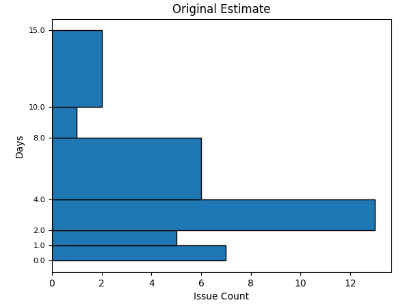
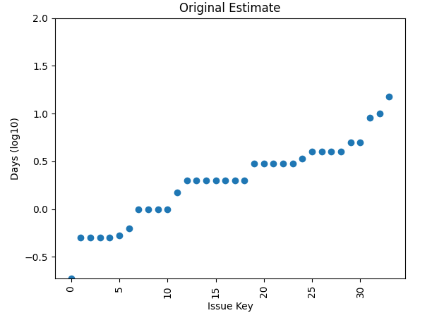
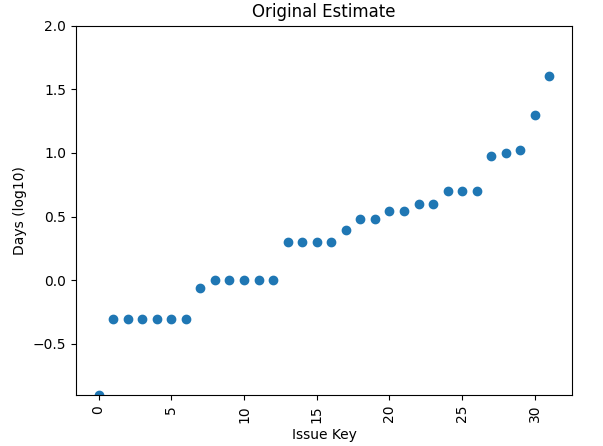
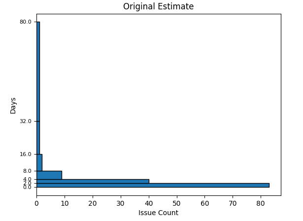
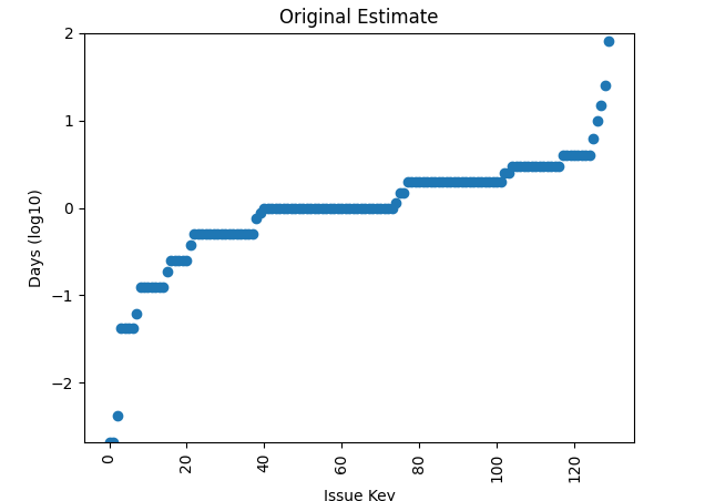
The following plots depict the original estimates for multiple projects. The plots on the left are histograms. Those on the right are sorted and with their \(log_{10}\) values plotted.

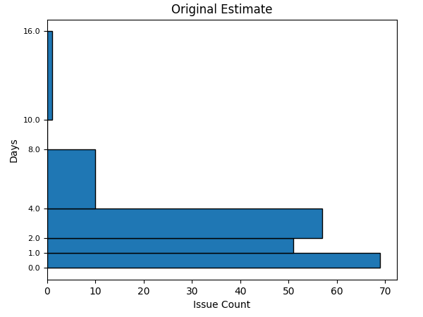
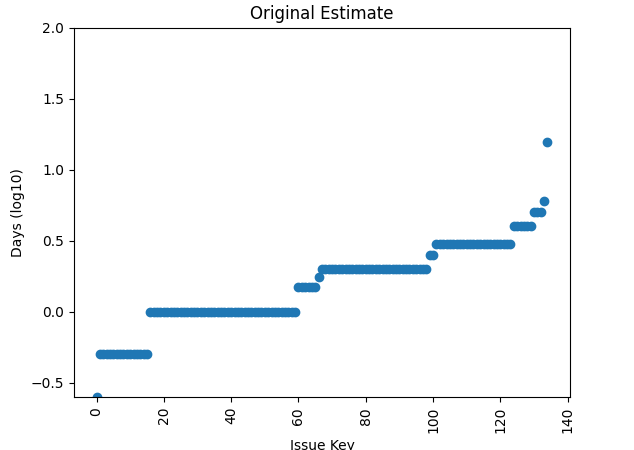
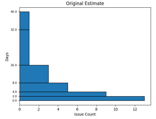
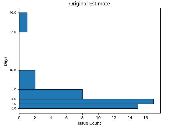
These plots use the original estimate for each task. If you are familiar with JIRA, this is not the sum of the original estimates. The sum hides important information about how the estimates are created. If I used the sum the layers in the right column would be less pronounced or nonexistent.

Is there a difference between estimating a 10 day task or two 5 day sub-tasks? I’ll argue yes. Intuitively, it seems likely that better estimates are possible for smaller tasks, but not always.

What do these plots tell me about the quality of our estimates? They tell me there is a tendency to gravitate to a few values \(\le 0\) and \(\le 10\). This range is closer to 0.3 days through to 8 days, which is evidenced in the histograms.

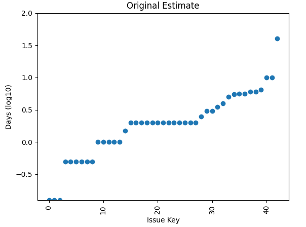
This trend gets even more pronounced using plot all of the data from all projects, as shown in the plot below.

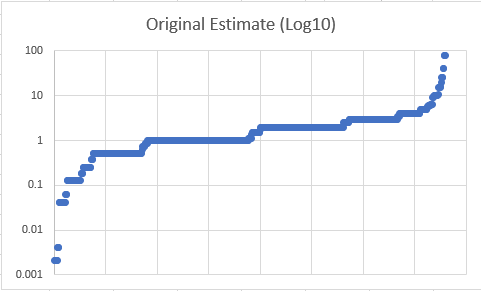
Here, it looks like the dominate plateaus are 0.5, 1, 2 and 5 days.

So these estimates tend to cluster in plateaus that tend to fall on durations of a week. Individual projects tend to have the same plateaus but it looks like these fall into 0.5, 1, 2 and 5 day ranges.