I’ve recently come across some comments by Michael Feathers relating to unconditional code. The basic idea is that that code containing lots of if-statements or nested if-statements should be viewed with suspicion. He extends this suspicion to switch-statements and loops.

It’s an incredibly powerful idea.

One concept he discusses to eliminate if-statements in a function is to look at error conditions and consider expanding the domain of the function to eliminate the error condition. I mentioned this to a couple of collegues and both asked what that means. I assume that domain refers to the function inputs (just like the mathematical definition of a function over a domain and range).

If I apply this meaning to a function the is seemingly nonmathematical in nature what can I come up with?

Here’s some Python code from Pandas that creates a Pandas data frame from a CSV file.

pandas.read_csv(file_handle, usecols = [ 'Index', 'Column One' ], index_col = [ 'Index' ], parse_dates = [ 'Index' ])

What’s interesting about this function is that it will accept CSV file containing only the header row (defined by usecols). The data frame created by this read_cvs under these conditions is empty. Nothing unreasonable about this.

If my application uses this function and goes off to compute something it needs to handle the case when no data is present gracefully. If my application just counted rows if data, I could achieve this by producing a count of zero. The point being that zero is as reasonable an answer as one, two or three if this is the number of rows present.

The problem with this example is that it’s not clear I’ve extended the domain of the count function.

If my application computes the average value of a column in this file then things get more interesting. Using the above example, I get a count of 0 rows and my data value is undefined (because it doesn’t exist).

Pandas deals with this very gracefully. Run read_csv on a CSV file containing only the header column and you can use pandas.isna on a column value to determine if the value is unavailable. My average calculation now needs to be aware of this situation and we can check for this situation using a count or pandas.isna. This awareness is likely to come in the form of an if-statement.

This brings me back to the initial question of how to extend the domain of my average calculator in the absence of any column values. In Michael’s example, he introduces the concept of a null object that participates in a computation but essentially does nothing.

In my average calculator, my average function should understand and operate on empty data frames by returning the equivalent of pandas.isna == True for the array. If it does, then the domain of the average function includes the any numeric value and “NA”. My application doesn’t contain an if-statement for this extended domain. It lives somewhere and that’s ok.

The point Michael is making, is that lots of if-statements are generally a bad sign. The total elimination of them is not.

Check out the Anti-If Campaign.

My team has a problem. They don’t disagree with each other or with me. They would rather go with the flow than rock the boat. This results in wasted effort and frustration.

The ability to respectfully disagree is an important trait of a healthy team. Nay, it’s a critical behaviour for a team to remain healthy.

Without disagreement there isn’t honest discussion. Without honest discussion nothing gets resolved.

Our lack of disagreement manifests in a few ways.

• Engaged team members would work on things the team said they needed. That work would be ignored. In one instance, a team member tried to support another by getting people to use the shared work. That activity ended in frustration.

• Our team meetings, modelled on Lean Coffee, don’t work. The only barrier to entry for Lean Coffee is having a topic you want to discuss. Or interest in what others have to say.

  First, the team couldn’t get the meeting to work because the meeting didn’t have enough structure. What were we trying to accomplish? How do we know what’s happening they asked. (I publish minutes with actions and dates.)

  People came to the meeting who didn’t know why they were there or what they wanted from it. There wasn’t anything they felt compelled to discuss. Nothing to share–no learnings, no process changes, no challenges. Nothing.

• Implict power relationships that manifest in terms of knowledge hoarding. Senior developers unable or unwilling to share with junior developers. Also manifested with people saying they weren’t involved in decisions they needed to know about.

People didn’t respect each other’s time or effort. Good ideas die a slow death of neglect after completion.

I misunderstood the difficulty with the team meeting because I focused on the barrier to entry. I think structure was an attempt to create a safe place to discuss important topics. But those who wanted the discussion were afraid.

When I first joined this team, the senior people weren’t engaged with the junior people. The junior people were frustrated and complained of not being able to learn things. This initially confused me because the dialog was all around the logistics of setting up a “lunch and learn”. Someone said the lack of pizza is an impediment to their learning.

I think of the pizza issue as a different form of a failure to disagree. Senior developers made excuses to cover disinterest and the junior developers naively accepted these excuses as legitmate. The junior developers settled. No pizza justified not investing in themselves.

For a while, I identified lack of disagreement as “not caring”. I asked why don’t you care about this topic or that. My notion of “caring” is simple: if you care you have an opinion or make a positive contribution to the issue. Team members argued they cared. Their arguments for “caring” never focused on the topic. They deflected it by pointing out how hard they were working.

Conversations are like this:

“We should do X to solve Y.”

“But X won’t solve Z.”

“What do you propose?”

“I’m not saying X won’t work.”

…

Classic argument: your idea doesn’t solve an adjacent problem and no alternatives are provided. Then retreat leaving confusion–should we be fixing Y or Z?

These arguments oppose change, hide a lack of support and try to discourage it. This isn’t very different from a Concern Troll. Introduce fear, uncertainty and doubt to create paralysis. Enshrine a do-nothing attitude wrapped in the platitudes of generating better outcomes.

I recognize failure to disagree as a lack of trust. My notion of caring implied debate, disagreement, decisions and commitment. The team’s interpretation of caring is that they were doing their jobs.

If you are a student of The Five Dysfunctions of a Team then improve trust by going first. The idea for creating conflict is to mine for it. I’m wearing a miner’s hat, light on and digging for the motherlode. Maybe get in some spelunking while I’m at it.

I’ve said a lot about working agreements (Working Agreements for Agile Teams (Part 6)). Good agreements are concise and easy to evaluate regarding whether they are being fulfilled or not and are unambiguous. Recently, I find myself reconsidering my position on ambiguity. Or at least a little ambiguity.

The team and I are facing challenges improving our test regime. One team member put forth the notion that it isn’t sufficient to test the product. We must use meaningful tests.

They defined meaningful tests using an example involving a histogram and bin counting. Their example went like this:

• we have a bin counting algorithm in our software.
• Bin counting describes a frequency distribution (like you’d see if you plotted a histogram of the counts).
• Any reasonable test must test the properties of a frequency distribution.

I’ll call this an argument for POLA. And think it reasonble.

The flaw in this argument is that it doesn’t describe a use case. For example, if I’m counting inventory and my bins are part numbers. It’s not clear this use case requires my bin counting algorithm to exhibit any property except retaining a count of parts for a given part number. A frequency distribution in this case might be useful but it might not be.

The difference is in how the information will be used–maybe I need to display a histogram, maybe I don’t.

In any event, the comment on developing meaningful tests piqued my interest. What is a meaningful test?

There isn’t one answer to this. I can argue that meaningful requires viewing bin counting through the lens of a frequency distribution. I can argue that it requires understanding the use case. I’m in the use case camp.

Since meaningful means different things to different people its use in the working agreement was ambigous. It’s ambiguous because I can easily check if you wrote a test. The meaningfulness of any test is debatable without a shared understanding of the requirement.

I’m confident the team will eventually come around to the realization that meaningful tests provide evidence the requirement is fulfilled. This will remove the ambiguity.

In the meantime, the use of meaningful in our working agreement is ambiguous because of different interpretations of what a meaningful test is. It’s power might also come from the realization that you can’t debate meaningful without a shared understanding of the outcome.

The power of ambiguity in a working agreement is exploration required to remove the ambiguity. A little ambiguity is, in effect, a powerful learning tool for an engaged team.

One aspect of my current position involves working with 3D models. I’m curious about the data structures used to model 3D objects and why polygons and triangles are used in these models. ¹

The first representation was developed in 1972 by Bruce G. Baumgart: Winged-edge Polyhedron Representation. It includes a body, face, edge and vertex polyhedron for modelling objects.

A polyhedron:

A “polyhedron” in algebraic topology is defined as a space that can be built from “building blocks” such as line segments, triangles, tetrahedra, and their higher dimensional analogs by “gluing them together” along their faces.

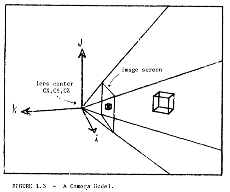
The paper describes a way of mapping between the “real world” and the “model world”. The interface between these worlds is a camera that constructs a 2-dimensional image of the 3-dimensional world it views.

This article walks through Part I of the Winged-edge Polyhedron Representation. The diagrams below are from the original paper.

The Model World

The model world is made of addressable content (essentially computer memory). It comprises:

• topological data which includes the notion of neighbourhood. The face, edge and vertex are essentially part of surface topology. Volume topology is computed. (Topology refers to the geometric surface characteristics of a 3D object.)
• geometric data which includes the notion of locus, length, area and volume. (A locus is a set of all points (e.g., a line, a line segment, a curve or surface), whose location satisfies or is determined by one or more conditions.)
• photometric data which includes the notion of locus, light source and data on light absorbed, reflected, or refracted from the surface.
• parts tree data which descibes the notion that object are composed of parts in the physical world (and not how the entity is broken into parts).

Addressing mechanisms via access requirements.

• appearance uses camera coodinates to show what the world looks like through that camera.
• recognition return model world objects that are present in the image.
• camera solution use image coordinates to determine camera coodinates in real world.
• perception use camera solution to place bodies in image that are not yet recognized.
• spatial accessing given a locus and radius return portion of objects in that sphere.

Camera Model

The Real World

Real-world coordinates:

• Camera lens centre: \(CX\), \(CY\) and \(CZ\).
• Camera frame of reference: with unit vectors \(I\), \(J\), \(K\) form a right-handed coordinate system.
• Rotation matrix: \[\begin{array}{cc} IX & IY & IZ \\
  JX & JY & JZ \\
  KX & KY & KZ \end{array} \]
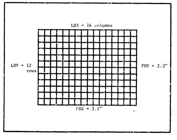
• Scales determining correspondence between real-world and image size.
  • Logical raster size: \(LDX\), \(LDY\) and \(LDZ\). The integer LDZ is an artifact so the units come out correctly in the Z dimension.

  • Physical raster size: \(PDX\), \(PDY\) and \(FOCAL\), where \(FOCAL\) is the focal plane distance. In this model, the focal plane distance is equated with the lens focal length. ²

    \(SCALEX \leftarrow -FOCAL \times \frac{LDX}{PDX}\) \(SCALEY \leftarrow -FOCAL \times \frac{LDY}{PDY}\) \(SCALEZ \leftarrow FOCAL \times LDZ\)

Body, Face, Edge and Vertex (BFEV) Modelling

Vertex

A vertex is a point in Euclidean space. It has world locus and world-coordinates \((XWC, YWC, ZWC).\) They are the basic data from which area, volume, face vectors and image positions are calculated.

A vertex may exist simultaneously in multiple image spaces.

An image space with perspective-projected coordinates \((XPP, YPP, ZPP)\). Perspective-projected coordinates are always 3-dimensional and determined with respect to a given camera-centred coordinate system \((XCC, YCC, ZCC)\). The perspective-projected frame is right handed.

The tranformation of a vertex world locus to a camera centred locus is as follows.

• Translation to the camera frame’s origin: \[\begin{array}{ccc} X & \leftarrow & XWC - CX \\
  Y & \leftarrow & YWC - CY \\
  Z & \leftarrow & ZWC - CZ \end{array} \]

• Rotation to the camera frame’s origin: \[\begin{array}{ccc} XCC & \leftarrow & IX \times X + IY \times Y + IZ \times Z \\
  YCC & \leftarrow & JX \times X + JY \times Y + JZ \times Z \\
  ZCC & \leftarrow & KX \times X + KY \times Y + KZ \times Z \\
  \end{array} \]

• Perspective projection transformation. \[\begin{array}{ccc} XPP & \leftarrow & SCALEX \times \frac{XCC}{ZCC} \\
  YPP & \leftarrow & SCALEY \times \frac{YCC}{ZCC} \\
  ZPP & \leftarrow & \frac{SCALEZ}{ZCC} \end{array} \]

  \(XPP\) and \(YPP\) are derived by means of similar triangles.

  \(ZPP\) is always taken inversely proportional to the distance of the vertex from the camera image plane \(ZCC\). It preserves depth and collinearity of the world in the perspective-projected image space.

Vertices in front of the camera’s image plane have negative \(ZPP\). \(ZPP\) values near \(-FOCAL\) are close to the camera; those near zero are far away.

The valence of a vertex is the number of edges that meet at a vertex.

Edge

An edge can be thought of as two vertices. These edges define the 2-dimensional line coefficients.

\[\begin{array}{cc} AA & \leftarrow & Y1 - Y2 \\
BB & \leftarrow & X2 - X1 \\
CC & \leftarrow & X1 \times Y2 - X2 \times Y1 \end{array} \]

The coefficients appear in the 2-dimensional equation of the line containing the edge: \(0 = AA \times X + BB \times Y + CC\).

When the edge coefficents are normalized: \[\begin{array}{cc} L & \leftarrow & \sqrt{AA + 2 + BB + 2} \\
AA & \leftarrow & \frac{AA}{L} \\
BB & \leftarrow & \frac{BB}{L} \\
CC & \leftarrow & \frac{CC}{L} \end{array} \]

The distance from the line to a point \((X, Y)\) is \(Q \leftarrow \lvert AA \times X + BB \times Y + CC \rvert\).

Determining if two edges intersect:

• First, check if the end points of one edge are in the opposite half planes of the other edge.
• Second, check if the end points of the latter edge are in the opposite half planes of the first edge.

If both conditions are true then:

\[\begin{array}{cc} T & \leftarrow & (A1 \times B2 - A2 \times B1) \\
X & \leftarrow & \frac{(B1 \times C2 - B2 \times C1)}{T} \\
Y & \leftarrow & \frac{(A2 \times C1 - A1 \times C2)}{T} \end{array} \]

Check for the identity case.

Check for edges with a common vertex.

Face

A face is a finite region of plane enclosed by straight lines. Faces have characteristice coeeficients: \(AA \times A + BB \times Y + CC \times ZZ = KK\).

\(AA\), \(BB\) and \(CC\) are unit normal vectors. \(KK\) is the distance of the origin from the plane.

The coefficent of a plane can be computed using Cramer’s rule. ³ \[\begin{array}{cc} KK & \leftarrow & X1 \times (Z2 \times Y3 - Y2 \times Z3) \\
& & + Y1 \times (X2 \times Z3 - Z2 \times X3) \\
& & + Z1 \times (Y2 \times X3 - X2 \times Y3) \\
AA & \leftarrow & (Z1 \times (Y2 - Y3) + Z2 \times (Y3 - Y1) + Z3 \times (Y1 - Y2) \\
BB & \leftarrow & (X1 \times (Z2 - Z3) + X2 \times (Z3 - Z1) + X3 \times (Z1 - Z2) \\
CC & \leftarrow & (X1 \times (Y3 - Y2) + X2 \times (Z3 - Z1) + X3 \times (Y2 - Y1) \end{array} \]

Normalized:

\[\begin{array}{cc} ABC & \sqrt{AA + 2 + BB + 2 + CC + 2} \\
AA & \frac{AA}{ABC} \\
BB & \frac{BB}{ABC} \\
CC & \frac{CC}{ABC} \\
KK & \frac{KK}{ABC} \end{array} \]

If vertices \(V1\), \(V2\) and \(V3\) are taken counter clockwise around the exterior of the solid then the relations obtain:

• \(AA \times X + BB \times Y + CC \times Z \le KK\) implies \(X\), \(Y\) and \(Z\) are above the plane.
• \(AA \times X + BB \times Y + CC \times Z = KK\) implies \(X\), \(Y\) and \(Z\) are in the plane.
• \(AA \times X + BB \times Y + CC \times Z \ge KK\) implies \(X\), \(Y\) and \(Z\) are below the plane.

Face coefficents are useful in world and image coordinate systems.

Polyhedra, Bodies and Objects

Simple polyhedra satisfy Euler’s equation \(F - E + V = 2\). A simple polyhedron is one homemorphic to a sphere. Euler’s equation is the primitive basis of the data structure.

A body is an entity more specific than a polyhedron. A polyhedron is represented by the whole structure of bodies, faces, edges and vertices.

A body may have a location, orientation and volume in space. It be connected to faces, edges and vertices which may or may not form a complete polyhedron.

The number of polyhedra associated with a body varies depending upon the object being represented. An object refers to physical objects (e.g., a tree).

A single body is often associated with one polyhedra when representing a rigid object (e.g., a sledge hammer). Several bodies are often associated with one polyhedra when representing a flexible object (e.g., a human being).

The body is also used to represent parts and abstract regional objects (e.g., hierachical composites). For example, a parking lot comprises isles, lanes and lamp islands. A lamp island comprises a lamp; a lamp has a base and top.

The parts structure is carried in body nodes.

Four Kinds of BFEV Accessing

1. Accessing by name and serial number. Involves retreival using a symbolic name.

2. Parts-Tree Accessing. Occurs between different bodies.

   At the top of the world exists a body to which all other bodies are attached. Given a body, a list of sub-parts and it’s supra-part can be accessed.

   A supra-part is the whole entity to which a part belongs. The world is its own supra-part.

3. FEV Sequence Accessing.

   Each body provides sequential accessing to each face, edge and vertex. Sequential access is required because

   • perpsective projection loops through every vertex.
   • display clipping loops through all edges.
   • body intersection loops through all faces.

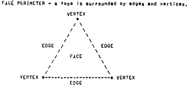
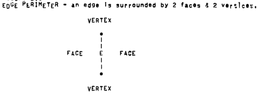
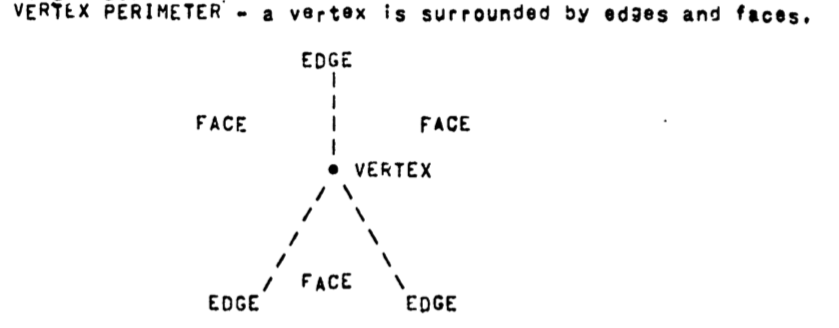
4. FEV Perimeter Accessing.

   Perimeter accessing requires that given a face, edge or vertex the perimeter of that entity be readily accessible:

   • faces have a perimeter of edges and vertices.

• edges have a perimeter of two faces and two vertices.

• vertices have a perimeter of edges and faces.

The surface of a polyhedron is orientable (has a well defined inside and outside). This means perimeter lists can be ordered (say clockwise) with respect to the polyhedron’s exterior.

Footnotes

^{1. The introduction: “It is my current predjudice that polyhedra provide the proper starting point for building a physical world representation.” But are they really triangles? In face, “A safe formal face structure could be built by defining a triangle as three non-colinear vertices and insisting that all faces be triangle interiors.”, but the implementation may be different. ↩}

^{2. Under what circumstances does focal length differ from focal distance? Some hints: Ray Optics. ↩}

^{3. The original document refers to Kramer’s rule. Apparently, a typo. ↩}

I’ve had occasion to write some tools that explore ticket data using JIRA. JIRA provides a rich REST API for doing these kinds of explorations.

One of the problems I ran into was the concept of worklog. JIRA associates a worklog with each JIRA issue.

The basic relationship is that a project is associated with zero or more issues. Each issue is associated a worklog. Each worklog has zero or more worklogs (I’ll call these worklog entries to differentiate them from the issue worklog).

My problem was finding a good class breakdown for this structure. I started by focusing on the collections of worklogs associated with a project.

The code looked something like this:

Worklog = namedtuple('Worklog', 'created comment timeSpentSeconds')

class IssueWorklog(object):
    def __init__(self, issue_key):
        self._worklog = list(map(lambda worklog: Worklog._make(worklog['created'], worklog['comment'], worklog['timeSpentSeconds']), GetIssueWorklog(issue_key)

    def get_worklog_entry(self):
        for worklog in self._worklog:
            yield worklog

class ProjectWorklog(object):
    def __init__(self, project_key):
        self._worklog = list(map(lamda issue: IssueWorklog(issue['key']), SearchUri(project_key)))

    def get_worklog_entry(self):
        for worklog in self._worklog:
            yield worklog

(GetIssueWorklog() and SearchUri() are methods that manages calls to the Get Issue Worklog and Search resources defined in JIRA’s REST API.)

Needless to say, I hated this implementation. I hated it because the use of classes in this instance is overkill. All this does is create a collection of worklog entries.

Other parts of my applications took the worklog entries and generated plots from them. In all, you could do this with three functions (or a nested for-loop):

  For each issue in the project:
     For each worklog entry in the issue:
         Add worklog entry to a container.

In my opinion, I’ve completely missed the point of good design.

An alternative design that I like much better looks like this.

WorklogEntry = namedtuple('WorklogEntry', 'created comment timeSpentSeconds')

class ResampleFrequency(Enum):
    MONTH_END = 'M'

class Worklog(object):
    """A collection of worklog entries from a project, an issue, or both."""

   def __init__(self, worklog_entries):
       self._df = pd.DataFrame(sorted(worklog_entries, key = lambda worklog: worklog.created), columns = WorklogEntry._fields)

   def doSumAndResample(self, new_frequency):
       return self._df.resample(new_frequency).sum(), columns = [ 'timeSpentSeconds'])

The important part here is the shift in emphasis from operations for the collection of worklog entries to operations on WorklogEntry objects. Here a worklog entry is a container and the Worklog class does all of the heavy lifting.

Can I do better than the doResampleAndSumTimeSeries() method? Well, let’s see.

# Worklog information collected from a JIRA issue.
WorklogEntry = namedtuple('Worklog', 'key summary comment created timeSpentSeconds')

class ResampleFrequency(Enum):
    """Enumerate different Pandas resample freqencies using Pandas DateOffset objects."""
    MONTH_END = 'M'

class Worklog(object):
    """Construct a Panda data frame from collected worklogs.

    A worklog can be viewed as a time series depicting time spent, along with other metadata.
    """
    def __init__(self, worklog_entries: List[WorklogEntry]):
        """Construct the worklog object using the provided worklog entries."""
        df = pd.DataFrame.from_records(sorted(worklog_entries, key = lambda worklog: worklog.created), columns = WorklogEntry._fields)
        self._df = df.set_index(pd.DatetimeIndex(pd.to_datetime(df['created'], utc = True)))

    def doResampleAndSumTimeSeries(self, resample_frequency: ResampleFrequency):
        """Resample and sum the worklog's time spent values using the provided resample frequency."""
        self._df = pd.DataFrame(self._df.resample(resample_frequency.value).sum(), columns = [ 'timeSpentSeconds' ])

    def doCalculateRollingAverage(self, window_size: int):
        """Caclulate a rolling average of the worklog's time spent values."""
        self._df['rollingAverageTimeSpentSeconds'] = self._df.rolling(window = windw_size).mean()

    def doMakeDataFrame(self) -> pd.DataFrame:
        """Make a data frame from the worklog object."""
        return self._df

It’s not perfect. It’s not perfect because I wrap the Pandas data frame with operations that manipulate the JIRA worklogs. It provides an advantage in that the maniplation of the data frame is contained within the class. It has the disadvantage of exporting the data frame which seems disappointing in terms of extending the class.