Recently, I needed to create a database using Qt. I used How to embed a database in your application with SQLite and Qt by Davide Coppola to get started. My experiment involved mimicking database migrations in Diesel. My needs are more modest and I used C++.

A database migration involves executing queries to alter the database structure of a live application so the schema contains what the application expects. It’s useful for application upgrades (and downgrades).

Imagine you have an application, App and that App version 1 (v1) is deployed. When v2 is deployed, there are two important use cases to handle. Assume that v2 contains database schema changes (e.g., v2 might require a table column that doesn’t exist in v1).

1. A new user installs v2. This experience should be identical to a user installing v1. This user has no data and should be able to install and use the application immediately.

2. An existing user upgrades from v1 to v2. This experience should be identical to installing v1 but it’s likely that they have information they want to keep in their existing database. Since the database schema has changed you need a way to update the database structure to the revision required by v2.

   It is this situation where the notion of a database migration is helpful. In a migration you write the SQL statements to move from database schema, revision 1 to revision 2 and execute them. This get more interesting when moving from v1 to higher a version, say v3, v5 or v10.

The idea provided in Diesel is to write queries for up- and down- grading the database schema by creating SQL statements that change the schema or table structure. My example only supports schema upgrades. It’s also assumes upgrading from App, v1, schema revison 1 to the current schema revision.

The essential idea is to recognize that a database schema is a whole-part hierarchy and that the Composite design pattern might be ideal to represent it.

In my implementation, the Component (Schema) is a base class to the Leaf (TableRevision) and the Composite (TableRevisionHistory).

The TableRevisionHistory contains a vector of TableRevisions that are executed in the order they are created by the migrate() method. Following the execution of migrate() the database structure reflects the lastest revision of the schema.

The Schema interface. The database is a parameter and not a state variable because the schema state does not depend upon a database.

class Schema // Component
{
public:
    virtual ~Schema() = 0;
    virtual const bool migrate(Database&) = 0;

protected:
    Schema() noexcept;
};

A table revision contains only the SQL statement defining the revision. A better choice for the SQL statement type might be q QSqlQuery or a QString. Using the definition of an SQL statement below has the advantage of keeping Qt dependencies out of this class.

class TableRevision // Leaf
    : public Schema
{
public:
    typedef const char *sql_statement_type;

    TableRevision(sql_statement_type s)
        : sql_statement(s) { }

    ~TableRevision() { }
    virtual const bool migrate(Database&) override;

private:
    sql_statement_type sql_statement; // The SQL statement used to revise the table structure.
};

To define a table and create a revision. Strictly speaking I don’t need a table revision class (e.g., table could inherit directly from schema). Its presence conveys the intent of the pattern more clearly.

class Table
    : public TableRevision
{
public:
    typedef TableRevision::sql_statement_type sql_statement_type;

    Table(sql_statement_type s)
        : TableRevision(s) { }

    ~Table() { }
};

Table revision0("CREATE TABLE people (id INTEGER PRIMARY KEY, name TEXT)");

The table revision history interface.

class TableRevisionHistory
    : public Schema
{
public:
    typedef Schema* value_type; //!< Schema container value type.
    typedef std::unique_ptr<value_type> pointer_type;  //!< Schema pointer type.
    typedef std::vector<pointer_type> container_type;  //!< Schema container type.

    virtual ~TableRevisionHistory();
    virtual const bool migrate(Database&) override;
    virtual void add(value_type);

protected:
    TableRevisionHistory();

private:
    container_type revision_history;
};

Schema revision isn’t supported explicitly. It’s implied by the number of table revisions stored in the table revision history. This was a surprise, as I thought revision would be part of the schema state.

One way to manage schema revision is to use a database table metadata that includes schema revision information. For example, table could the current revision of each table (e.g., the highest index used during the last update). An upgrade would require that the ‘migrate()’ begin it’s migration at the metadata revision’s plus one.

Another issue with schema revision is how to store it given that there are any number of tables whose revisions might all be different. It seems there is a lot calculation (e.g., schema revision is the sum of all table revisions) or a maintenance issue (e.g., hard coded revision number). Neither approach is strictly necessary.

To add an entry to the revision history.

class TableHistory
    : public TableRevisionHistory
{
public:
    /*! @brief Create the table history object.
     */
    TableHistory()
        : TableRevisionHistory() { }

    /*! @brief Destroy the table history object.
     */
    ~TableHistory() { }
};

TableHistory history;
history.add(&revision0);
if(history.migrate(database)) {
  return true;
}
else {
    return false; // Handle error.
}

Of course, you could managed the revision history any number of ways. A simple vector would suffice. The advantage of using the Composite pattern is the client can use the same interface regardless of the number of tables or the number of revisions of those table.

The source code.

In Data Measurement and Analysis for Software Engineers, I go through Part 3 of a talk by Dennis J. Frailey. Part 3 looks at statistical techniques for data analysis in software engineering and takes a look at normal and non-normal statistics. In this article, I look at Part 4 of the webinar. Part 4 covers statistical techniques for data analysis that are well suited for software.

Descriptive statistics are used to describe, show or summarize data in a visual way that is meaningful. They are also known as robust statistics. They are not developed using probability theory but may rely in inferential statistics.

Descriptive statistics include central tendency, median, mean and mode and measures of variability. Variability includes standard deviation, variance, minimum and maximum. (And only when these statistics are meaningfully supported by the scale.)

Graphs are commonly used to enhance descriptions. They include:

• box plots
• bar charts and histograms
• control charts
• scatter charts and correlation

Box Plots

Box plots are useful for showing median and quartile information for quantitative information. They are useful whenever the data is not on a ratio scale or is not normally distributed. The data must be on an ordinal scale or higher. Box plots are good for showing normal and unusual conditions.

Box plots are used for a comparison. They are used on an irregular basis.

Bar Charts and Histograms

A histogram plots a distribution of data using bars to represent mode for a particular element of the data. Order is important, so the bars cannot be reordered.

A bar chart is used to plot categorical data and can be reordered. They are used to compare values.

A Pareto chart is a bar chart where the bars are ordered from largest to smallest and a line chart is used to generate totals. An interesting review of the statistical basis (and an improvement) is available from Revising the Pareto Chart.

Control Charts

A control chart is used to track the performance of a process or a machine. It shows actual data against average data in comparision to expected variation (the control limits). The average and expected variation are based upon previous data or projects.

If historical data is unavailable, assume the data is normally distributed.

A control chart tells you when a process or machine is performing outside of its normal limits and shows when to take action. A good example for using control charts with software processes is available as quantitative software management and related CMMI processes.

Control charts are used for tracking a regular basis. Use them to see how things change over time and to spot trends.

Correlation

An exploration of whether different variables are related. Correlation is not causation.

Popular methods of correlation.

• Pearson coefficent for normal data.
• Spearman coefficent for non-normal data. It is computed on the rank of data and answers the question regarding whether the data can be described using a monotonic function.
• Kendall coefficent for non-normal data.
• Regression uses an equation to determine if there is a relationship.

Spearman and Pearson are measures of association.

In McCall’s Software Quality Model I take a look at McCall’s Software Quality Framework. Here, I explore the concept of Testabilty in this framework as a means of improving software quality. McCall defines Testability as

Effort required to test a program to ensure it performs its intended function.

Effort is measured in terms of time, cost (dollars), or people and is the subject of Managing Cost in McCall’s Quality Model. How to ensure a program fulfills its intended function is another matter entirely.

Intuitively, good testing provides confidence in the correct operation of a program.

Testability is a measure of the degree a program supports testing. (See Software Testability for another definition.) Ensuring a program fulfills its intendend function is a different factor.

McCall’s definition of Testability includes criterion to ensure ease of testing.

• simplicity: avoid practices that increase complexity.
• modularity: introduce practices that promote highly independent modules (focus on high cohesion and low coupling).
• instrumentation: measure usage and error identification.
• self-descriptiveness: provide explanations of the functions performed by the software.

These criterion don’t ensure intended function because they don’t explicitly address it. The intuitive notion of correct operation isn’t part of Testability. It’s part of Correctness.

The Correctness quality factor is defined as

Extent to which a program satisfies its specifications and fulfills the user’s mission objectives.

Fortunately, Testability is improved by focusing on factors that positively affect it. Graphically, this looks like:

This graphic uses the rows and columns for Correctness and Testability in Tables 4.2-2 and 4.2-3 of Factors in Software Quality. The criterion are from Table 4.1-1 in the same document.

All factors depicted here positively affect Testability and Correctness. Several criteria positively affect Testability. The intuitive notion of whether a program fulfills its intended function lies in the traceability, completeness and consistency criterion. Only the traceability and consistency criterion positively affect Testability.

In fact, traceability is defined as

Those attributes of the software that provide a thread from the requirements to the implementation with respect to the specific development and operational environment.

and consistency as

Those attributes of the software that provide uniform design and implementation techniques and notation.

Testability is enabled by the factors linked to it but its definition is fulfilled by traceability between requirements and implementation. Traceabilty creates a closed-loop that provides confidence the tests test the program’s intended function.

Traceability relies on cross referencing related modules to requirements (through the design and implementation phases at the system level). The model suggests a traceabiltiy matrix be used for this.

However, traceability is insufficient to for Testability. It is insufficient because traceability doesn’t ensure all requirements are covered in both design and system test.

Traceability is defined as the total number of requirements traced divided by the total number of requirements. This is achieved by

1. using design to identify the requirements statisfied by a module.
2. using implementation to identify the requirements statisfied by a module’s implementation.

Ensuring that the total number of requirements traced is fulfilled by the completeness criteria. Completeness ensures, among other things, that

• the design agrees with the requirements and
• the code agrees with design.

Completeness is defined as

Those attributes of the software that provide full implementation of the functions required.

Completeness create a closed-loop between requirements and implementation by leveraging traceability. Is consistency needed? It’s defined as

Those attributes of the software that provide uniform design and implementation techniques and notation.

Consistency relies upon explicitly employing conventions that aid completeness and traceability. The interplay between consistency, completeness and testability ensure a program fulfills its intended function.

If I want to employ Testability metrics I need to deploy mechanisms that measure the criterion supporting it. I also need to employ metrics for Correctness and, very likely, factors defined by quality criteria identified as positively affecting Testability.

In all, Testability relies on eight direct or indirect criterion and six factors. If you want testable code you can’t focus on just Testability. This fact emphasizes one of the great points of this quality model: quality is a lifecycle activity.

In Data Measurement and Analysis for Software Engineers, I go through Part 2 of a talk by Dennis J. Frailey. Part 2 looks at basic analysis techniques for software engineering and what makes a good measurement process. In this article, I look at Part 3 of the webinar. Part 3 covers statistical techniques for data analysis.

Perhaps the most valuable information in Part 3 is the discusson on dealing with normal and non-normal sets of data. Most software metrics result in sets of data that are not on a normal distribution. Most common statistical techniques assume a normal distribution. Misapplying statistical techniques leads to a variety of errors.

In what follows, I highlight the most important elements from the webinar including:

• Statistics for normal distributions of data including:
  • Central Tendency Measures,
  • Measures of Dispersion and
  • Confidence Intervals and Confidence Levels.
• Challenges involving software metrics including:
  • Types of Studies,
  • Hypothesis Testing and
  • Exploring Relationships.
• Choosing an Evaluation Technique including Techniques for Non-Normal Distributed Data.

Normally Distributed Statistics

Software metrics may not contain normally distributed data. This section includes a description of the statistic and caveats for identifying when not to use them.

Central Tendency Measures

A measure of central tendency is

a single value that attempts to describe a set of data by identifying the central value within that set of data.

These are the

• mean (the average of all data values),
• median (the middle data value) and
• mode (the most frequent data value).

If these values are all equal it suggests, but does not guarentee, that the set of data has a normal distribution. The potential for skew in data makes it critically important to pay attention to the distribution in the data.

If the values are positively skewed then \(mode > median > mean.\) If negatively skewed then \(mean < median < mode.\) If positive or negative skew is present the mean will not identify the middle value. The median will.

The mode can be

• undefined (all values occur equally),
• bimodal (there are two most frequent values) and
• multimodal (there are multiple most frequent values).

Bimodal and multimodal data sets occur whenever there are several local maximums.

The mode can be computed for any scale (i.e., nominal, ordinal, interval and absolute scales). The median requires at least an ordinal scale; the mean requires at least a ratio scale. Most software metrics rely upon ordinal scales, so only the median and mode are applicable.

Measures of Dispersion

A measure of dispersion is

a single value that attempts to descibe a set of data by identifying the spread of values within that set of data.

The most common measures of dispersion are

• the range. It is the distance between the largest and smallest values in the set of data. It requires an interval scale to compute.
• the variance. It is a measure of how far the numbers are spread out. It is particularly useful when looking at probability distributions. A variance of zero means the numbers are all the same; a small variance means the numbers are close together and a large variance means they are not.
• the standard deviation. It is a value used to represent the amount of variation or dispersion in a set of data. In a normally distributed set of data each standard deviation is the same size (or the same distance from the mean).

Variance and standard deviation both require a ratio scale.

Confidence Intervals and Confidence Levels

A confidence interval is

a range of values that have a strong chance of containing the value of an unknown parameter of interest.

A confidence level is

a probability that a value will fall within the confidence interval.

A margin of error is

normally half the confidence interval.

Using continuous functions to approximate data requires understanding confidence intervals and levels.

Conclusions are valid only if the confidence level is high (\(95\%\)). Such levels usually have narrow confidence intervals. A wide interval means the data includes a wide range of values. A wide range means variance is high. High variance is often a problem with software metrics.

Software Metrics

A challenge with metrics is the presence of uncontrolled variables. They require that information be evaluation using

• available information or
• through your own study.

A challeng with available information is that they are just opinion. In the worst case, they are exagerations. A challenge with software engineering studies is that they are not easily reproduced or are reproduced only a small number of times.

Don’t draw conclusions using poorly designed studies.

Types of Studies

A study looks at data. It provides evidence for a hypothesis but not proof. The purpose of a study is to

1. test or confirm a hypothesis or theory.
2. explore a relationship.

By comparision, an experiement generates data. To properly establish cause and effect, an experiment must be repeated independently many times. If the hypothesis can be independently verified by many experiments, then it becomes a theory. A theory is a possible explanation for observed behaviour that accurately predicts the phenomena.

Hypothesis Testing

A hypothesis is a possible explanation of an observed phenomenon. The goals of a hypothesis are to explain a phenomenon and to predict the consequences. To test a hypothesis conduct an experiment to evaluate cause and effect.

A hypothesis speculates that given certain values of some independent variables we can predict the values of dependent variables. Independent variables are controlled (changed) to study their effect on dependent variables.

In hypothesis testing there may be

• many variables,
• variables that are not controllable or
• confounding effects between variables.

Examples of confounding variables include the environment, tools, processes, capabilities of people and application domain.

Uncontrolled and confounding variables may affect the outcome of any study or measurement. The more of these variables the less reliable the results.

We can evaluate evidence by asking

• does the evidence support the hypothesis?
• how likely does it support the hypothesis by chance?

A test of significance is a measure of how likely the results are due to chance. In classical statistics, significance means there is a \(95\%\) confidence level that the hypothesis is true. This confidence level is difficult to show if the data is widely dispersed.

To test or confirm a hypothesis use an analyis of variations (ANOVA):

• test two or more methods, tools, etc.
• use statistical tests to determine the differences and see if they are statistically significant.

If the differences are statistically significant the hypothesis might be right–there is empirical evidence for the difference. If not, then the hypothesis is probably wrong.

A statistical significance result provides support for a hypothesis. It does not prove it.

Errors that might show statisitically significant results, even when the hypothesis is incorrect include

• experimental errors.
• the presence of uncontrolled variables.
• the presence of confounding variables.
• use of an invalid statistical technique.

Statistical techniques commonly used for ANOVA.

• Student’s T Test,
• F Statistics and
• Kruskal-Wallis and other advanced techniques.

Exploring Relationships

Exploring relationships is best done using robust statistics. Robust statistics include graphs, charts and diagrams. Approaches used include

• box plots (summarizes the range and distribution of data for a single variable),
• bar charts (compares a small number of entities),
• control charts (shows trends and abnormalities over time),
• scatter diagrams (shows the relationship between two variables) and
• correlation analysis (statistical methods to supplement scatter diagrams).

Choosing an Evaluation Technique

The major considerations when choosing an evaluation technique.

• the nature of the data. This includes consideration of
  • the relationship of the set of data to the larger population.
  • the distribution of the set of data. Many statistical techniques assume normally distributed data.
  • the scale of the set of data.
• the purpose of the study. This could be to confirm a theory or hypothesis or to explore a relationship.
• the study design. Identification and use of the best techniques to support the purpose of the study.

The sample size is important because many statistical techniques compare the relative sample size to the population size to suggest a confidence interval. Other considerations are whether the sample is truly a random selection. A larger sample size generally improves confidence. So does running multiple experiments.

Many statistical techniques assume

• the variables are independent.
• the observations are independent.
• there are no controlled or confounding variables.
• all data is described using an interval or ratio scale.
• that the dependent variable is related to the independent variable by a linear function.
• independence of experiments (i.e., one experiement does not influence the other).
• outliers have no significant effect on the mean and median.

Good technique requires that you test your assumptions prior to using the technique.

Ways to contaminate normally distributed data

• by contamination with bad data. Even 1-5 percent of bad data can render statistical techniques invalid.
• by mixing two more more normally distributed datasets that have difference means, medians or modes.
• small departures in the assumptions described above.

Techniques for Non-Normal Distributed Data

For non-normal distributed data

• determine the underlying distribution and apply techniques suitable for that distribution.
• change the scales.
• use nonparametric statistical methods.

Nonparametric methods do not use parameterized families of probability distributions. They tend to be used on populations of ranked data and may not need mean, median or variance. (Data ranked using ordinal scales.)

The are used on two main categories of data

• descriptive statistics. A descriptive statistic (in the count noun sense) is a summary statistic that quantitatively describes or summarizes features of a collection of information. A descriptive statistics in the mass noun sense is the process of using and analyzing those statistics. It is solely concerned with properties of the observed data, and it does not rest on the assumption that the data come from a larger population.
• inferential statistics. Inferential statistical analysis infers properties of a population, for example by testing hypotheses and deriving estimates. It is assumed that the observed data set is sampled from a larger population.

In Data Measurement and Analysis for Software Engineers, I discuss the first of four webinars on measurment by Dennis J. Frailey. A key point in the first webinar is the importance of understanding the scales used for measurement and the statistical techniques usable on those scales.

Here, I take a look at scales of measurement and Stanley S. Stevens’ article On the Theory of Scales of Measurement. Stevens was interested in measuring auditory sensation. I’m interested in defect severity. Both measures have some surprising commonality.

Stevens defines measurement as

the assignment of numerals to objects or events according to rules.

Stevens wanted to measure the subjective magnititude of auditory sensation against a scale with the formal properties of other basic scales. Basic scales include those used to measure weight and length.

The rationale for Stevens’ focus on scales of measurement was the recognition that

• rules can be used to assign numerals to attributes of an object.
• different rules create different kinds of scales for these attributes.
• different scales create different kinds of measurement on these attributes.

These differences require definition of

1. the rules for assigning measurement,
2. the mathematical properties (or group structure) of the scales and
3. the statistcal operations applicable to each scale.

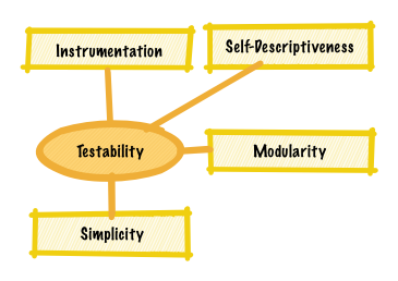
Rules for Specifying Severity

Defect severity is an example of an ordinal scale. An ordinal scale includes:

• rules for specifying severity.
• the properties of a nominal scale for severity, that permit
  • contigency correlation for severity and
  • hypothesis testing of defect severity. This scale has properties that permit the determination of equality.
• the properties of an ordinal scale for severity. These properties permit the determination of greater or less than.

An example where rules are needed is the determination of the severity of a defect. Without rules, severity level reflects the reporter’s intuitive notion of severity. This notion is likely to differ by reporter and possibly by the same reporter over time.

Rules ensure that different reporters consistently apply severity level to defects. Consistently applying severity level ensures that all defects have the same scale of severity. Using the same scale means the mathematical properties of that scale are known. This permits determination of the applicable statistical operations for severity.

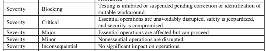
The focus on rules is a response to the subjective nature of the measurement. Defect severity is a subjective measure, as shown by the definition of severity (see IEEE Standard Classification for Software Anomalies):

The highest failure impact that the defect could (or did) cause, as determined by (from the perspective of) the organization responsible for software engineering.

This standard defines the following severity levels.

Importantly, this definition seeks a scale of measure that reflects a common prespective of severity. This common perspective is created using severity level and shared notions of essential operation and of significant impact.

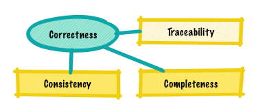
The Properties of a Nominal Scale for Severity

Severity has the properties of a nominal scale. A nominal scale uses numerals (or labels) to create different classes. Stevens’ calls this a nominal scale of Type B. A Type B nominal scale supports the mode (frequency) and hypothesis testing regarding the distribution of cases amongst different classes and contengency correlation.

A hypothesis test might use severity from all releases to determine if overall quality has improved. To be meaningful, this test would require the same rules for assigning severity applied to each release included in the test.

Contigency Correlation for Severity

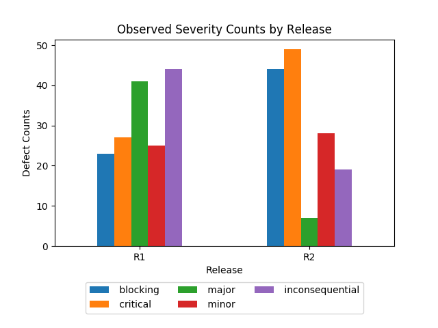
An example of contengency correlation for defects by release uses two categorical variables: Release and Severity. Release has 2 cases (i.e., R1 and R2); Severity has 5 cases (i.e., Blocking through Inconsequential).

Releases R1 and R2 (the most recent release) have these observed defect counts by severity:¹

Release	Blocking	Critical	Major	Minor	Inconsequential	Total
R1	23 (14.4%)	27 (16.9%)	41 (25.6%)	25 (15.6%)	44 (27.5%)	160 (52.1%)
R2	44 (29.9%)	49 (33.3%)	7 (4.8%)	28 (19.0%)	19 (12.9%)	147 (47.9%)
Total	67 (21.8%)	76 (24.8%)	48 (15.6%)	53 (17.3%)	63 (20.5%)	307 (100.0%)

Observed characteristics:

• The totals provide the observed frequency of each severity level using the last two releases. That is, the frequency of Blocking severities is \(67\) out of \(307\) observations.
• The mode severity is Inconsequential, Blocking and Critical for R1, R2 and R1 and R2, respectively.

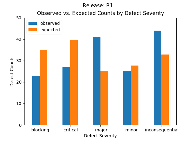
Releases R1 and R2 have the following expected defect counts by severity:²

Release	Blocking	Critical	Major	Minor	Inconsequential	Total
R1	34.9 (21.8%)	39.6 (24.8%)	25.0 (15.6%)	27.6 (17.3%)	32.8 (20.5%)	160 (100.0%)
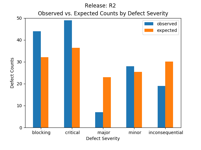
R2	32.1 (21.8%)	36.4 (24.8%)	23.0 (15.6%)	25.4 (17.3%)	30.2 (20.5%)	147 (100.0%)
Total	67.0 (21.8%)	76.0 (24.8%)	48.0 (15.6%)	53.0 (17.3%)	63.0 (20.5%)	307 (100.0%)

Expected characteristics:

• All expected values are normalized using the frequencies in the total row of the observed table.
• The severity frequency is Critical for R1, R2 and R1 and R2, respectively.
• R1 has lower than expected Blocking, Critical and Minor severity counts than what is observed. Higher than expected in Major and Inconsequential than what is observed.
• R2 has lower than expected Major and Inconsequential severity counts than what is observed.

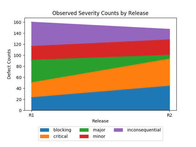
Graphically, these look like:

The expected values reflect a proportionality dictated by the frequency of the observations. The next section investigates whether this proportionality has any bearing on the observations.

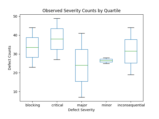
This figure depicts the same observations for R1 and R2 using a box plot.

A box plot shows the maximum and minimum values (the top and bottom crosses), along with the median value (middle of the box). The box top and bottom for the top and bottom 25 pecentiles of the data.

This box plot tells a story of very high Blocking and Critical defects in both releases. It conceals information on the individual releases, for example, has R2 improved?

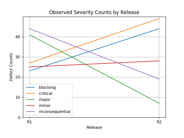
To understand if R2 is better than R1 the following graphs are helpful.

Clearly, R2 is worse than R1 in terms of the introduction of higher severity defects, despite the fact that the defect counts are smaller. (An area plot seems more informative than a stacked bar plot, but both provide the same information.)

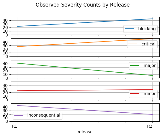
For more emphasis on individual severity counts. (These plots focus on individual severity counts and are less busy than the preceeding line chart.)

Hypothesis Testing on Severity Distributions

A nominal scale permits hypothesis testing of the distribution of the data. Severity is a form of categorical data. Categorical data is divided into groups (e.g., Blocking and Inconsequential).

There are several tests for the analysis of categorical data. The most appropriate one in this case, is the Categorical Distribution. A Categorical Distribution is a generalization of the binomial distribution, called a multinomial distribution.

A binomial distribution is a distribution where a random variable can take on only one of two values (i.e., \(0\) or \(1\)). The number of trials in a binomial is \(n = 1\). A Multinomial distribution where each trial can have an outcome in any one of several categories.

A Categorical Distribution is a vector of length \(k > 0\), where \(k\) is the number of elements in a vector were only one element has the value \(1\). The others have a value of \(0\). The number of trials in a Categorical Distribution is \(n = 1\).

Since a defect can have only one severity level, severity can be viewed as a vector with \(k = 5\) with only one vector element equal to \(1\). (I assume determining severity is a statistically independent event.⁴)

Statistically, we can use the expected severity to determine the probability for a distribution of severity counts. In the table above, the expected severity is a multinomial distribution.

The probability that these severity counts are \((67, 76, 48, 53, 63)\) is

\[\begin{align} \begin{array}{ccl} Pr(67, 76, 48, 53, 63) & = & \frac{307!}{67! \times 76! \times 48! \times 53! \times 63!}(0.218^{67} \times 0.248^{76} \times 0.156^{48} \times 0.173^{53} \times 0.205^{63}) \\ & = & 1.5432158498238714 \times 10^{-05} \\ \end{array} \end{align}\]

The probability of this severity count distribution is \(0.000015,\) or \(3\) in \(200000.\)

There are \(382,313,855\) discrete combinations of severity that sum to \(307.\) (The sum is a constraint placed upon the multinomial distribution, otherwise the probabilities fail to sum to \(1\).) Some statistics on this probability distribution, including counts by severity:

We want to test the null hypothesis \(H_{0}\) is the null hypothesis of homogenity. Homogenity implies that all probabilities for a given category are the same. If the null hypothesis fails, then at least two of the probabilities differ.

For this data set, the \(\chi^{2}\) parameters are as follows.

\[\begin{align} \begin{array}{lcr} \chi^{2} & = & 46.65746412772634 \\ \mbox{p-value} & = & 1.797131557103987e-09 \\ \mbox{Degrees of Freedom} & = & 4 \\ \end{array} \end{align}\]

The null hypoyhesis is rejected whenever \(\chi^{2} \ge \chi^{2}_{\alpha, t - 1}\). Clearly, the p-value, an indicator of the likelihood the results support the null hypothesis, is false. Two or more probabilities differ.

The 95% confidence intervals with \(\alpha = 0.05\) and \(Z_{1 - \alpha /2} = 1.96\) are computed: \[ p_{j} \pm Z_{1 - \alpha /2} \times \sqrt{\frac{p_{j} \times (1 - p_{j})}{n}}, \forall \, j, 0 \le j \le n. \]

The confidence intervals for each category are:³

\[\begin{align} \begin{array}{ccc} Blocking & = & 0.218 +/- 0.046 \\ Critical & = & 0.248 +/- 0.048 \\ Major & = & 0.156 +/- 0.041 \\ Minor & = & 0.173 +/- 0.042 \\ Inconsequential & = & 0.205 +/- 0.045 \\ \end{array} \end{align}\]

These values provide a confidence interval for each binomial in the multinomial distribution. They are derived using the “Normal Approximation Method” of the Binomial Confidence Interval.

Severity as an Ordinal Scale

Severity is referred to as an ordinal scale. Although it has nominal scale properties, it supports the properties of an ordinal scale. In effect the operations permitted on a scale are cumulatitve–any analysis supported by a nominal scale can be conducted on an ordinal scale.

This cumulative effect of scales is one of two major contributions made by this paper. The other being the definition of measurment itself. Isn’t that cool?

An ordinal scale permits determination of greater or less than–a Blocking defect is more severe than a Critical one. This is why we can say that R2 is worse than R1, despite the reduction in reported defects. There are more Blocking and Critical defects in R2 and these, because of the properties of an ordinal scale, are more severe than the others.

I don’t compute the median of severity in these releases because the distance between ordinals is unclear. Better to stick with frequency as it’s unambiguous.

References

The code used to generate the graphs: GitHub.

Footnotes

^{1. Severity counts randomly generated courtesy of RANDOM.ORG. R1 and R2 were generated by requesting 5 numbers in the range of 1 through 100, inclusive. ↩}

^{2. Each entry is calculated using the formula \(\frac{\mbox{row total} \times \mbox{column total}}{\mbox{table total}}\). ↩}

^{3. To make statistically valid conclusions a population of 301 is requred for a confidence interval of 1 and confidence level of 99%. This implies that this table is saying something significant regarding the observed severity in both release R1 and R2. ↩}

^{4. Is a defect severity a statistically independent event? It is because the severity of one defect does not influence the severity of any other defect. By contrast, defects are not independent events. For example, a defect in requirements that remains undetected until implementation will generate a collection of related defects. Is the severity of those related defects the same as the one identified in requirements or different? ↩}